Multidimensionale model with 3 dimensions-parameters
Data is generated: I my model I have 500 products, sold in 500 shops, in a 96 months time periode.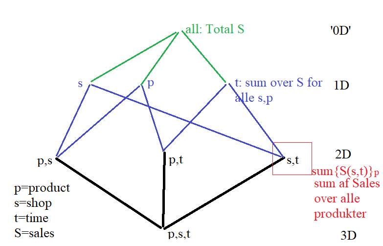
p0:0-499 ('Product'), p1:0-499 ('Shop/Location'), p2:0-95 (time: 'MonthNo); fact number is sales=sales values s.
3D table, the full table, fulltable_3D
has columns [p0, p1, p2, s], a row has data for sales s as a function of (p0,
p1, p2), i.e., the sales value for product p0 in shop p1 at time p2. The 96 p2
parameter values represent 96/12=8 years of monthly values. This gives 500*500*96=24 million rows.
I Regret I use symbols par0,par1,par2 for p0,p1,p2 and sum for s in the tables
I Use 3 smallint, 2B each, for the p's and 8B-double for s, so each row's data
occupies 3*2+8=14B, but there is a lot of overhead, in fact, the table occupies 828MB, with an average
of 37B per row.
I Create a Primary Index(p0, p1, p2), great for finding
sales for a specific combination of (p0, p1, p2) using
select sum from fulltable_3D where
p0=product[i], p1=shop[j], p2=time[k],
Data is then physically stored in order by (p0, p1,
p2); additionally, I create Index(p0), Index(p1), Index(p2), HashIndex(p0, p1)
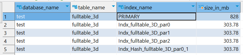
The 4 indices occupy 4*300MB, a
total of approx 828+1200=2.0GB
Here it would be smart to expand fulltable_3D with a 5th column with costs c,
the table would then perhaps occupy 2.3GB, with the same 4 indices. Similarly, the 2D and
1D tables described below can be expanded with an extra c-column.
SELECT database_name, table_name, index_name,
ROUND(stat_value * @@innodb_page_size / 1024 / 1024, 2) size_in_mb
FROM mysql.innodb_index_stats
WHERE stat_name = 'size' and table_name LIKE 'fulltable_3d'
ORDER BY size_in_mb DESC;
2D table, p2D(p for parameter space in 2D, besides table name as 2D is not allowed)
gives variation over 2 parameters, with summation over the 3rd parameter. Made as one table, it is simple, but gives some null spaces:
|par0 |par1 |par2 |s
Null 0 0 sum{s(i,0,0)}i sum over 500 par0-values, with i-indeks
Null 0 1 sum{s(i,0,1)}i
.. .. .. .. 500*96=48000 rows
0 Null 0 sum{s(0,j,0)}j sum over 500 p1-values, j indeks,
0 Null 1 sum{s(0,j,1)}j
500*96=48000 rows
.. .. .. ..
0 0 Null sum{s(0,0,k)}k sum over 96 p2-values, k-indeks,
0 1 Null sum{s(0,1,k)}k 500*500=250000 rows
.. .. .. ..
The table has a total of 250000+296*500 =346000 rows, the table occupies 13.5MB. I Create 3 indices,
one for each column p0-p2 and indices with pairs of parameters and
Hash-index(par0,par2); table and indices occupy a total of about 42MB
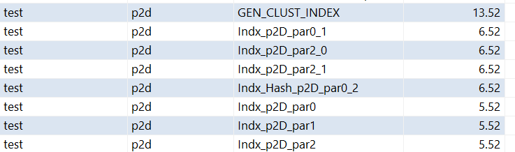
Index: 4*6.52+3*5.52=42.6MB
Version 2 of the 2D table is a better choice/modeling:
e.g., p2D_par01, with columns [par0, par1, sum]
|par0 |par1 |s
0 0 sum{s(0,0,i)}i sum over 96 p2-values,
0 1 sum{s(0,1,i)}i 500*500=250000 rows
..
Where e.g., sum{s(0,1,i)}i is sale for product 0, in
shop 1, summed over all periods, the total sale
And similarly p2D_par02 with columns [par0, par2,
sum{s(par0,i,par2)}i] and p2D_par12 with columns [par1, par2,
sum{s(i,par1,par2)}i ], these two have 50096=48000
rows
In total, the three tables have 346000 rows like the first version. But it is a big advantage that
indexing is much more favorable, we can settle for one very efficient Primary
Index(pari, parj) in each table, where data is stored
physically in paramter-order. I have only created the largest p2D_par01, which
occupies 8.5MB with built-in Primary Index, so the three occupy probably
8+3+3=14MB
Best 10 shops for the best product (499) can be found using table p2D:
SELECT par1 as shop, sum FROM p2d where par0=499 and
par2=null order by sum desc ,
It is slow, I have tried all reasonable indexes.
It is calculated much faster with the table p2d_01:
SELECT par1 as shop, sum FROM p2d_01 where par0=499
order by sum desc , which only takes approx 5% of the calculation time for version
1,
see Best 10 shops for best product (499)-4
But p2D_01 is not good for the related problem: finding the best 10 products for the best
shop, here p2D is better to use!
Three 1D tables,
{p1D_j}j=0,1,2; in p1D_0 the value in row r is the summation over p1 and p2 for
p0=r, i.e., sum{s(r,i,j,)}i,j
The value in row r in table table 1D_2 is the sum of sales for all products and all shops at time r.
The 3 tables are small, only 500,500,96 rows, so the search through these is
lightning fast, I still create indexes for each table (it is created
automatically anyway). I create Primary Index on pj in each table.
I also have a Time dimension table, TimeDim(Year, Quarter, MonthInYear,
MonthNo)
with monthly resolution/granularity, MonthNo is the month number since the
start, 0-96 for 8 years. Parameter p2/par2 the 3D,2D,1D tables is key to MonthNo; it
corresponds to having stored monthly snapshots of sales (and possibly also costs c).
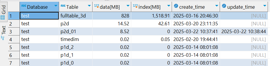
Information about each table and index size, mySQL:
SELECT
table_schema as `Database`,
table_name AS `Table`,
round(data_length / 1024 / 1024, 2) `data[MB]`,
round(index_length / 1024 / 1024, 2) `index[MB]`,
create_time,
update_time
FROM information_schema.TABLES where table_schema like 'test';
ORDER BY `data[MB]` DESC
Sum of sales for each month for the hole period:
select t.year,t.MonthNo,t.MonthInYear, p1.sum from timedim t,p1D_2 p1 where t.MonthNo=p1.par order by MonthNo , few milli sec(ms)
Total Sales for a Random Month
select sum as sum from p1D_2 where par=".$MonthNo (=random month)
where par2=MonthNo , few ms
Yearly total Sales
Methode 1
select distinct year,max(MonthNo) as max_MonthNo from timedim group by year
-> finds last MonthNo, max_MonthNo, i each year, then I calculate the accumulated sale op to each value of max_MonthNo
select sum(sum) as sum from p1D_2 where par<='max_MonthNo'
-> typical 5-10ms
Better Methode:
select sum(p1.sum) as sum,year from p1D_2 as p1, timedim as t where p1.par=t.MonthNo group by year order by year
Sum of Sales from 10 Best Products
select par as product, sum from p1D_0 order by sum desc few ms
from which, the first 10 product-id values
are extracted, saved in array $Products[]
Yearly Sales for Best Product ($Products[0]) Method 1:
Yearly sales for best product, $Products[0]
Method 1: First, max(MonthNo) for each year is found, then
accumulated sale up to year YearX can be found:
SELECT sum(sum) as sum FROM p2D where
par0=".$Products[0]." and par2<=".$max(MonthNo)YearX
Method 2 (20 times faster):
select sum(p2.sum) as sum, t.year from p2D as p2,
timedim as t where p2.par2=t.MonthNo and p2.par0=".$Products[0]."
group by t.year order by t.year
In both case I use the table p2D with (par0=$Products[0], par2=MonthNo )
Without using a multidimensional database model, I can use a table with all data, fulltable_3D
Here, the total sales for each product are found
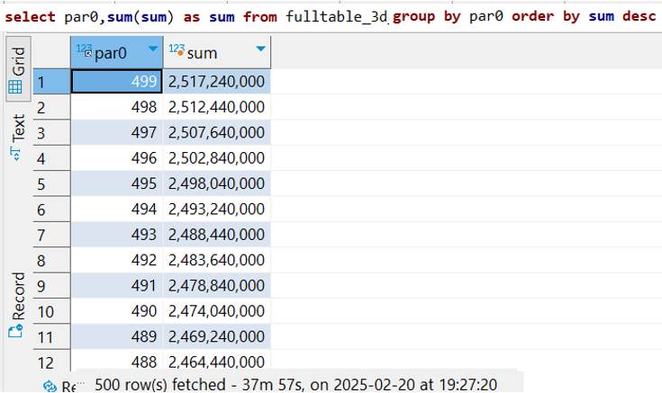
It takes 38 minutes! Useless in practice!
Sales for a Specific Product and Shop at a Specific Time
Sales at a specific 3D point (par0, par1, par2) are found, where par0=productId, par1=shopId, and par2=TimeId.
-use fulltable_3D:SELECT sum FROM $table where par0=$par0 and par1=$par1 and par2=$par2
gives sum of sales, a requst takes 1-2ms, quite good with 24 million rows. Here, the Primary Index on (par0, par1, par2) is used, not surprisingly.
If we want to calculate the sale for a specific product and shop within a time period, this can be used:
SELECT sum(sum) FROM $table where par0=$par0 and par1=$par1 and par2<=$par2 ,
Here, two indices are used: (index_par0,index_par1) to find rows with (par0, par1), which gives the 96 rows
with different par2[month values], which are then sequentially traversed (since we need to sum up over all par2 values).